{
"cells": [
{
"cell_type": "markdown",
"metadata": {},
"source": [
"\n",
"\n",
""
]
},
{
"cell_type": "markdown",
"metadata": {},
"source": [
"# Matplotlib\n",
"\n",
"\n",
""
]
},
{
"cell_type": "markdown",
"metadata": {},
"source": [
"## Contents\n",
"\n",
"- [Matplotlib](#Matplotlib) \n",
" - [Overview](#Overview) \n",
" - [The APIs](#The-APIs) \n",
" - [More Features](#More-Features) \n",
" - [Further Reading](#Further-Reading) \n",
" - [Exercises](#Exercises) \n",
" - [Solutions](#Solutions) "
]
},
{
"cell_type": "markdown",
"metadata": {},
"source": [
"## Overview\n",
"\n",
"We’ve already generated quite a few figures in these lectures using [Matplotlib](http://matplotlib.org/).\n",
"\n",
"Matplotlib is an outstanding graphics library, designed for scientific computing, with\n",
"\n",
"- high-quality 2D and 3D plots \n",
"- output in all the usual formats (PDF, PNG, etc.) \n",
"- LaTeX integration \n",
"- fine-grained control over all aspects of presentation \n",
"- animation, etc. "
]
},
{
"cell_type": "markdown",
"metadata": {},
"source": [
"### Matplotlib’s Split Personality\n",
"\n",
"Matplotlib is unusual in that it offers two different interfaces to plotting.\n",
"\n",
"One is a simple MATLAB-style API (Application Programming Interface) that was written to help MATLAB refugees find a ready home.\n",
"\n",
"The other is a more “Pythonic” object-oriented API.\n",
"\n",
"For reasons described below, we recommend that you use the second API.\n",
"\n",
"But first, let’s discuss the difference."
]
},
{
"cell_type": "markdown",
"metadata": {},
"source": [
"## The APIs\n",
"\n",
"\n",
""
]
},
{
"cell_type": "markdown",
"metadata": {},
"source": [
"### The MATLAB-style API\n",
"\n",
"Here’s the kind of easy example you might find in introductory treatments"
]
},
{
"cell_type": "code",
"execution_count": null,
"metadata": {
"hide-output": false
},
"outputs": [],
"source": [
"%matplotlib inline\n",
"import matplotlib.pyplot as plt\n",
"plt.rcParams[\"figure.figsize\"] = (10, 6) #set default figure size\n",
"import numpy as np\n",
"\n",
"x = np.linspace(0, 10, 200)\n",
"y = np.sin(x)\n",
"\n",
"plt.plot(x, y, 'b-', linewidth=2)\n",
"plt.show()"
]
},
{
"cell_type": "markdown",
"metadata": {},
"source": [
"This is simple and convenient, but also somewhat limited and un-Pythonic.\n",
"\n",
"For example, in the function calls, a lot of objects get created and passed around without making themselves known to the programmer.\n",
"\n",
"Python programmers tend to prefer a more explicit style of programming (run `import this` in a code block and look at the second line).\n",
"\n",
"This leads us to the alternative, object-oriented Matplotlib API."
]
},
{
"cell_type": "markdown",
"metadata": {},
"source": [
"### The Object-Oriented API\n",
"\n",
"Here’s the code corresponding to the preceding figure using the object-oriented API"
]
},
{
"cell_type": "code",
"execution_count": null,
"metadata": {
"hide-output": false
},
"outputs": [],
"source": [
"fig, ax = plt.subplots()\n",
"ax.plot(x, y, 'b-', linewidth=2)\n",
"plt.show()"
]
},
{
"cell_type": "markdown",
"metadata": {},
"source": [
"Here the call `fig, ax = plt.subplots()` returns a pair, where\n",
"\n",
"- `fig` is a `Figure` instance—like a blank canvas. \n",
"- `ax` is an `AxesSubplot` instance—think of a frame for plotting in. \n",
"\n",
"\n",
"The `plot()` function is actually a method of `ax`.\n",
"\n",
"While there’s a bit more typing, the more explicit use of objects gives us better control.\n",
"\n",
"This will become more clear as we go along."
]
},
{
"cell_type": "markdown",
"metadata": {},
"source": [
"### Tweaks\n",
"\n",
"Here we’ve changed the line to red and added a legend"
]
},
{
"cell_type": "code",
"execution_count": null,
"metadata": {
"hide-output": false
},
"outputs": [],
"source": [
"fig, ax = plt.subplots()\n",
"ax.plot(x, y, 'r-', linewidth=2, label='sine function', alpha=0.6)\n",
"ax.legend()\n",
"plt.show()"
]
},
{
"cell_type": "markdown",
"metadata": {},
"source": [
"We’ve also used `alpha` to make the line slightly transparent—which makes it look smoother.\n",
"\n",
"The location of the legend can be changed by replacing `ax.legend()` with `ax.legend(loc='upper center')`."
]
},
{
"cell_type": "code",
"execution_count": null,
"metadata": {
"hide-output": false
},
"outputs": [],
"source": [
"fig, ax = plt.subplots()\n",
"ax.plot(x, y, 'r-', linewidth=2, label='sine function', alpha=0.6)\n",
"ax.legend(loc='upper center')\n",
"plt.show()"
]
},
{
"cell_type": "markdown",
"metadata": {},
"source": [
"If everything is properly configured, then adding LaTeX is trivial"
]
},
{
"cell_type": "code",
"execution_count": null,
"metadata": {
"hide-output": false
},
"outputs": [],
"source": [
"fig, ax = plt.subplots()\n",
"ax.plot(x, y, 'r-', linewidth=2, label='$y=\\sin(x)$', alpha=0.6)\n",
"ax.legend(loc='upper center')\n",
"plt.show()"
]
},
{
"cell_type": "markdown",
"metadata": {},
"source": [
"Controlling the ticks, adding titles and so on is also straightforward"
]
},
{
"cell_type": "code",
"execution_count": null,
"metadata": {
"hide-output": false
},
"outputs": [],
"source": [
"fig, ax = plt.subplots()\n",
"ax.plot(x, y, 'r-', linewidth=2, label='$y=\\sin(x)$', alpha=0.6)\n",
"ax.legend(loc='upper center')\n",
"ax.set_yticks([-1, 0, 1])\n",
"ax.set_title('Test plot')\n",
"plt.show()"
]
},
{
"cell_type": "markdown",
"metadata": {},
"source": [
"## More Features\n",
"\n",
"Matplotlib has a huge array of functions and features, which you can discover\n",
"over time as you have need for them.\n",
"\n",
"We mention just a few."
]
},
{
"cell_type": "markdown",
"metadata": {},
"source": [
"### Multiple Plots on One Axis\n",
"\n",
"\n",
"\n",
"It’s straightforward to generate multiple plots on the same axes.\n",
"\n",
"Here’s an example that randomly generates three normal densities and adds a label with their mean"
]
},
{
"cell_type": "code",
"execution_count": null,
"metadata": {
"hide-output": false
},
"outputs": [],
"source": [
"from scipy.stats import norm\n",
"from random import uniform\n",
"\n",
"fig, ax = plt.subplots()\n",
"x = np.linspace(-4, 4, 150)\n",
"for i in range(3):\n",
" m, s = uniform(-1, 1), uniform(1, 2)\n",
" y = norm.pdf(x, loc=m, scale=s)\n",
" current_label = f'$\\mu = {m:.2}$'\n",
" ax.plot(x, y, linewidth=2, alpha=0.6, label=current_label)\n",
"ax.legend()\n",
"plt.show()"
]
},
{
"cell_type": "markdown",
"metadata": {},
"source": [
"### Multiple Subplots\n",
"\n",
"\n",
"\n",
"Sometimes we want multiple subplots in one figure.\n",
"\n",
"Here’s an example that generates 6 histograms"
]
},
{
"cell_type": "code",
"execution_count": null,
"metadata": {
"hide-output": false
},
"outputs": [],
"source": [
"num_rows, num_cols = 3, 2\n",
"fig, axes = plt.subplots(num_rows, num_cols, figsize=(10, 12))\n",
"for i in range(num_rows):\n",
" for j in range(num_cols):\n",
" m, s = uniform(-1, 1), uniform(1, 2)\n",
" x = norm.rvs(loc=m, scale=s, size=100)\n",
" axes[i, j].hist(x, alpha=0.6, bins=20)\n",
" t = f'$\\mu = {m:.2}, \\quad \\sigma = {s:.2}$'\n",
" axes[i, j].set(title=t, xticks=[-4, 0, 4], yticks=[])\n",
"plt.show()"
]
},
{
"cell_type": "markdown",
"metadata": {},
"source": [
"### 3D Plots\n",
"\n",
"\n",
"\n",
"Matplotlib does a nice job of 3D plots — here is one example"
]
},
{
"cell_type": "code",
"execution_count": null,
"metadata": {
"hide-output": false
},
"outputs": [],
"source": [
"from mpl_toolkits.mplot3d.axes3d import Axes3D\n",
"from matplotlib import cm\n",
"\n",
"\n",
"def f(x, y):\n",
" return np.cos(x**2 + y**2) / (1 + x**2 + y**2)\n",
"\n",
"xgrid = np.linspace(-3, 3, 50)\n",
"ygrid = xgrid\n",
"x, y = np.meshgrid(xgrid, ygrid)\n",
"\n",
"fig = plt.figure(figsize=(10, 6))\n",
"ax = fig.add_subplot(111, projection='3d')\n",
"ax.plot_surface(x,\n",
" y,\n",
" f(x, y),\n",
" rstride=2, cstride=2,\n",
" cmap=cm.jet,\n",
" alpha=0.7,\n",
" linewidth=0.25)\n",
"ax.set_zlim(-0.5, 1.0)\n",
"plt.show()"
]
},
{
"cell_type": "markdown",
"metadata": {},
"source": [
"### A Customizing Function\n",
"\n",
"Perhaps you will find a set of customizations that you regularly use.\n",
"\n",
"Suppose we usually prefer our axes to go through the origin, and to have a grid.\n",
"\n",
"Here’s a nice example from [Matthew Doty](https://github.com/xcthulhu) of how the object-oriented API can be used to build a custom `subplots` function that implements these changes.\n",
"\n",
"Read carefully through the code and see if you can follow what’s going on"
]
},
{
"cell_type": "code",
"execution_count": null,
"metadata": {
"hide-output": false
},
"outputs": [],
"source": [
"def subplots():\n",
" \"Custom subplots with axes through the origin\"\n",
" fig, ax = plt.subplots()\n",
"\n",
" # Set the axes through the origin\n",
" for spine in ['left', 'bottom']:\n",
" ax.spines[spine].set_position('zero')\n",
" for spine in ['right', 'top']:\n",
" ax.spines[spine].set_color('none')\n",
"\n",
" ax.grid()\n",
" return fig, ax\n",
"\n",
"\n",
"fig, ax = subplots() # Call the local version, not plt.subplots()\n",
"x = np.linspace(-2, 10, 200)\n",
"y = np.sin(x)\n",
"ax.plot(x, y, 'r-', linewidth=2, label='sine function', alpha=0.6)\n",
"ax.legend(loc='lower right')\n",
"plt.show()"
]
},
{
"cell_type": "markdown",
"metadata": {},
"source": [
"The custom `subplots` function\n",
"\n",
"1. calls the standard `plt.subplots` function internally to generate the `fig, ax` pair, \n",
"1. makes the desired customizations to `ax`, and \n",
"1. passes the `fig, ax` pair back to the calling code. "
]
},
{
"cell_type": "markdown",
"metadata": {},
"source": [
"## Further Reading\n",
"\n",
"- The [Matplotlib gallery](http://matplotlib.org/gallery.html) provides many examples. \n",
"- A nice [Matplotlib tutorial](http://scipy-lectures.org/intro/matplotlib/index.html) by Nicolas Rougier, Mike Muller and Gael Varoquaux. \n",
"- [mpltools](http://tonysyu.github.io/mpltools/index.html) allows easy\n",
" switching between plot styles. \n",
"- [Seaborn](https://github.com/mwaskom/seaborn) facilitates common statistics plots in Matplotlib. "
]
},
{
"cell_type": "markdown",
"metadata": {},
"source": [
"## Exercises"
]
},
{
"cell_type": "markdown",
"metadata": {},
"source": [
"### Exercise 1\n",
"\n",
"Plot the function\n",
"\n",
"$$\n",
"f(x) = \\cos(\\pi \\theta x) \\exp(-x)\n",
"$$\n",
"\n",
"over the interval $ [0, 5] $ for each $ \\theta $ in `np.linspace(0, 2, 10)`.\n",
"\n",
"Place all the curves in the same figure.\n",
"\n",
"The output should look like this\n",
"\n",
"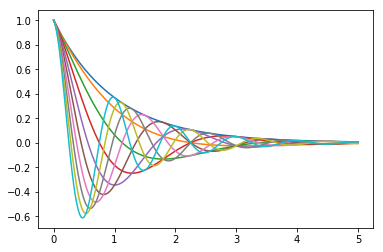"
]
},
{
"cell_type": "markdown",
"metadata": {},
"source": [
"## Solutions"
]
},
{
"cell_type": "markdown",
"metadata": {},
"source": [
"### Exercise 1\n",
"\n",
"Here’s one solution"
]
},
{
"cell_type": "code",
"execution_count": null,
"metadata": {
"hide-output": false
},
"outputs": [],
"source": [
"def f(x, θ):\n",
" return np.cos(np.pi * θ * x ) * np.exp(- x)\n",
"\n",
"θ_vals = np.linspace(0, 2, 10)\n",
"x = np.linspace(0, 5, 200)\n",
"fig, ax = plt.subplots()\n",
"\n",
"for θ in θ_vals:\n",
" ax.plot(x, f(x, θ))\n",
"\n",
"plt.show()"
]
}
],
"metadata": {
"date": 1614096162.8508897,
"filename": "matplotlib.md",
"kernelspec": {
"display_name": "Python",
"language": "python3",
"name": "python3"
},
"title": "Matplotlib"
},
"nbformat": 4,
"nbformat_minor": 4
}